Chapter 1
Basic Data Types
By Michael Castello
There are several different basic data types and it’s important to know what you can do with each of them so you can collect your data in the most appropriate form for your needs. People describe data types in many ways, but we’ll primarily be using the levels of measurement known as nominal, ordinal, interval, and ratio.
Levels of Measurement
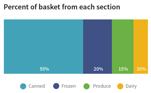
Let’s say you’re on a trip to the grocery store. You move between sections of the store, placing items into your basket as you go. You grab some fresh produce, dairy, frozen foods, and canned goods. If you were to make a list that included what section of the store each item came from, this data would fall into the nominal type. The term nominal is related to the Latin word “nomen,” which means “pertaining to names;” we call this data nominal data because it consists of named categories into which the data fall. Nominal data is inherently unordered; produce as a general category isn’t mathematically greater or less than dairy.
Nominal
Nominal data can be counted and used to calculate percents, but you can’t take the average of nominal data. It makes sense to talk about how many items in your basket are from the dairy section or what percent is produce, but you can’t calculate the average grocery section of your basket.
When there are only two categories available, the data is referred to as dichotomous. The answers to yes/no questions are dichotomous data. If, while shopping, you collected data about whether an item was on sale or not, it would be dichotomous.

Ordinal
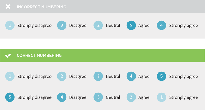
At last, you get to the checkout and try to decide which line will get you out of the store the quickest. Without actually counting how many people are in each queue, you roughly break them down in your mind into short lines, medium lines, and long lines. Because data like this has a natural ordering to the categories, it’s called ordinal data. Survey questions that have answer scales like “strongly disagree,” “disagree,” “neutral,” “agree,” “strongly agree” are collecting ordinal data. No category on an ordinal scale has a true mathematical value. Numbers are often assigned to the categories to make data entry or analysis easier (e.g. 1 = strongly disagree, 5 = strongly agree), but these assignments are arbitrary and you could choose any set of ordered numbers to represent the groups. For instance, you could just as easily decide to have 5 represent “strongly disagree” and 1 represent “strongly agree.”

Like nominal data, you can count ordinal data and use them to calculate percents, but there is some disagreement about whether you can average ordinal data. On the one hand, you can’t average named categories like “strongly agree” and even if you assign numeric values, they don’t have a true mathematical meaning. Each numeric value represents a particular category, rather than a count of something.
On the other hand, if the difference in degree between consecutive categories on the scale is assumed to be approximately equal (e.g. the difference between strongly disagree and disagree is the same as between disagree and neutral, and so on) and consecutive numbers are used to represent the categories, then the average of the responses can also be interpreted with regard to that same scale.
Interval
Enough ordinal data for the moment… back to the store! You’ve been waiting in line for what seems like a while now, and you check your watch for the time. You got in line at 11:15am and it’s now 11:30. Time of day falls into the class of data called interval data, so named because the interval between each consecutive point of measurement is equal to every other. Because every minute is sixty seconds, the difference between 11:15 and 11:30 has the exact same value as the difference between 12:00 and 12:15.
Interval data is numeric and you can do mathematical operations on it, but it doesn’t have a “meaningful” zero point – that is, the value of zero doesn’t indicate the absence of the thing you’re measuring. 0:00 am isn’t the absence of time, it just means it’s the start of a new day. Other interval data that you encounter in everyday life are calendar years and temperature. A value of zero for years doesn’t mean that time didn’t exist before that, and a temperature of zero (when measured in C or F) doesn’t mean there’s no heat.
Ratio
Seeing that the time is 11:30, you think to yourself, “I’ve been in line for fifteen minutes already…???” When you start thinking about the time this way, it’s considered ratio data. Ratio data is numeric and a lot like interval data, except it does have a meaningful zero point. In ratio data, a value of zero indicates an absence of whatever you’re measuring—zero minutes, zero people in line, zero dairy products in your basket. In all these cases, zero actually means you don’t have any of that thing, which differs from the data we discussed in the interval section. Some other frequently encountered variables that are often recorded as ratio data are height, weight, age, and money.
Interval and ratio data can be either discrete or continuous. Discrete means that you can only have specific amounts of the thing you are measuring (typically integers) and no values in between those amounts. There have to be a whole number of people in line; there can’t be a third of a person. You can have an average of, say, 4.25 people per line, but the actual count of people has to be a whole number. Continuous means that the data can be any value along the scale. You can buy 1.25 lbs of cheese or be in line for 7.75 minutes. This doesn’t mean that the data have to be able to take all possible numerical values – only all the values within the bounds of the scale. You can’t be in line for a negative amount of time and you can’t buy negative lbs of cheese, but these are still continuous.
To review, let’s take a look at a receipt from the store. Can you identify which pieces of information are measured at each level (nominal, ordinal, interval, and ratio)?
| Date: 06/01/2014 Time: 11:32am | ||||
|---|---|---|---|---|
| Item | Section | Aisle | Quantity | Cost (US$) |
| Oranges—Lbs | Produce | 4 | 2 | 2.58 |
| Apples—Lbs | Produce | 4 | 1 | 1.29 |
| Mozzarella—Lbs | Dairy | 7 | 1 | 3.49 |
| Milk—Skim—Gallon | Dairy | 8 | 1 | 4.29 |
| Peas—Bag | Frozen | 15 | 1 | 0.99 |
| Green Beans—Bag | Frozen | 15 | 3 | 1.77 |
| Tomatoes | Canned | 2 | 4 | 3.92 |
| Potatoes | Canned | 3 | 2 | 2.38 |
| Mushrooms | Canned | 2 | 5 | 2.95 |
Variable Type Vs. Data Type
If you look around the internet or in textbooks for info about data, you’ll often find variables described as being one of the data types listed above. Be aware that many variables aren’t exclusively one data type or another. What often determines the data type is how the data are collected.
Consider the variable age. Age is frequently collected as ratio data, but can also be collected as ordinal data. This happens on surveys when they ask, “What age group do you fall in?” There, you wouldn’t have data on your respondent’s individual ages – you’d only know how many were between 18-24, 25-34, etc. You might collect actual cholesterol measurements from participants for a health study, or you may simply ask if their cholesterol is high. Again, this is a single variable with two different data collection methods and two different data types.
There general rule is that you can go down in level of measurement but not up. If it’s possible to collect the variable as interval or ratio data, you can also collect it as nominal or ordinal data, but if the variable is inherently only nominal in nature, like grocery store section, you can’t capture it as ordinal, interval or ratio data. Variables that are naturally ordinal can’t be captured as interval or ratio data, but can be captured as nominal. However, many variables that get captured as ordinal have a similar variable that can be captured as interval or ratio data, if you so choose.
| Ordinal Level Type | Corresponding Interval/Ratio Level Measure | Example |
|---|---|---|
| Ranking | Measurement that ranking is based on | Record runners’ marathon times instead of what place they finish |
| Grouped scale | Measurement itself | Record exact age instead of age category |
| Substitute scale | Original measurement the scale was created from | Record exact test score instead of letter grade |
It’s important to remember that the general rule of “you can go down, but not up” also applies during analysis and visualization of your data. If you collect a variable as ratio data, you can always decide later to group the data for display if that makes sense for your work. If you collect it as a lower level of measurement, you can’t go back up later on without collecting more data. For example, if you do decide to collect age as ordinal data, you can’t calculate the average age later on and your visualization will be limited to displaying age by groups; you won’t have the option to display it as continuous data.
When it doesn’t increase the burden of data collection, you should collect the data at the highest level of measurement that you think you might want available later on. There’s little as disappointing in data work as going to do a graph or calculation only to realize you didn’t collect the data in a way that allows you to generate what you need!
Other Important Terms
There are some other terms that are frequently used to talk about types of data. We are choosing not to use them here because there is some disagreement about their meanings, but you should be aware of them and what their possible definitions are in case you encounter them in other resources.
Categorical Data
We talked about both nominal and ordinal data above as splitting data into categories. Some texts consider both to be types of categorical data, with nominal being unordered categorical data and ordinal being ordered categorical data. Others only call nominal data categorical, and use the terms “nominal data” and “categorical data” interchangeably. These texts just call ordinal data “ordinal data” and consider it to be a separate group altogether.
Qualitative and Quantitative Data
Qualitative data, roughly speaking, refers to non-numeric data, while quantitative data is typically data that is numeric and hence quantifiable. There is some consensus with regard to these terms. Certain data are always considered qualitative, as they require pre-processing or different methods than quantitative data to analyze. Examples are recordings of direct observation or transcripts of interviews. In a similar way, interval and ratio data are always considered to be quantitative, as they are only ever numeric. The disagreement comes in with the nominal and ordinal data types. Some consider them to be qualitative, since their categories are descriptive and not truly numeric. However, since these data can be counted and used to calculate percentages, some consider them to be quantitative, since they are in that way quantifiable.
To avoid confusion, we’ll be sticking with the level of measurement terms above throughout the rest of this book, except in our discussion of long-form qualitative data in the survey design chapter. If you come across terms “categorical,” “qualitative data,” or “quantitative data” in other resources or in your work, make sure you know which definition is being used and don’t just assume!